Efficient Connected Components Labeling for PyTorch

Some AI tasks sometimes require a post-processing step known as Connected Components Labeling (CCL). This can, for instance, be the case in certain Computer Vision tasks that involve segmentation (such as text or object detection).

To the best of my knowledge, there is no library that allows this to be done efficiently on GPU with PyTorch. Kornia offers a solution, but this implementation seems rather inefficient to me (multiple iterations on convolutions). Another unmaintained implementation exists, but it also doesn't work in batches, doesn't support images with odd dimensions and is not compatible with the latest versions of CUDA (and therefore PyTorch). There may be other workarounds out there, but I haven't found anything convincing.

So, I thought it would be cool to tinker with something a bit more sustainable (and I had fun learning some new stuff, so it's a win-win). Here, we'll explore the implementation of a (near) state-of-the-art approach for CCL on GPU. This implementation is available in the TorchCC library. The distribution of the package is still a bit shaky, but I'll try work on it.

GitHub - Bendabir/torchcc: Efficient Connected Components Labeling for PyTorch.

Efficient Connected Components Labeling for PyTorch. - Bendabir/torchcc

GitHubBendabir

Connected Components Labeling

Obviously, I’ve dug deep into the topic, so I more or less understand what I’m talking about, but I’ll try to introduce it briefly for those who are just joining.

Connected Components Labeling (CCL) is an algorithm used to identify and label groups of connected pixels in a binary image, where all the pixels in a group share the same value and are adjacent to each other. The way we define adjacency is key, but we'll get back to that later. By assigning unique labels to each connected region, the algorithm helps in isolating distinct objects or features within an image. On CPU, CCL is pretty straightforward, but scaling it efficiently on GPU requires some clever optimizations to handle parallelism and memory access.

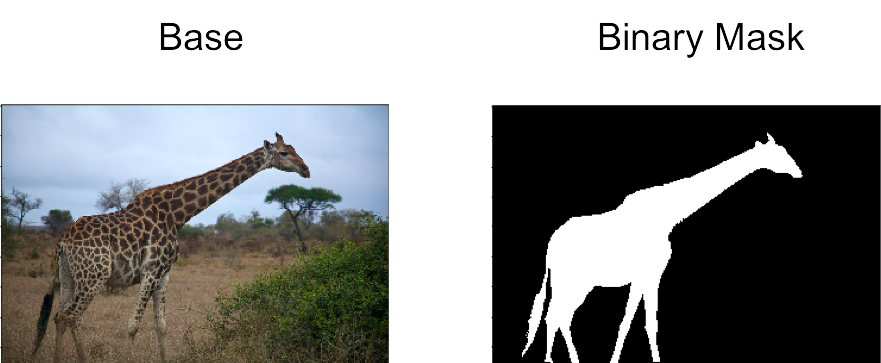
For instance, during a segmentation task, the model will generally produce a mask. In the case of object detection, the pixels representing an object will have a value of 1, while all other pixels will be set to 0. For text detection, the pixels containing text would be assigned the value 1 (no kidding).

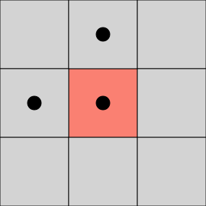
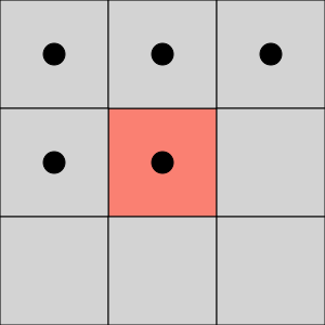
As explained earlier, a unique ID is assigned to groups of adjacent pixels. This adjacency can be defined either along the edges of the pixels only (4-connectivity), or along both the edges and corners (8-connectivity). In the following examples, the pixels marked by a black dot belong to the same connected component (based on the type of connectivity).

The Block-based Union-Find Algorithm

The Block Union-Find (BUF) algorithm is described by Allegretti et al. It aims to improve performances for 8-connectivity CCL. It can be extended to 3D cases (thus with 26-connectivity).

According to Bolelli et al., the Block-based Komura Equivalence (BKE), also described in Allegretti et at., is stlighty more efficient in general cases. It can also generalize to 3D. However, despite very similar, I found the BKE algorithm slightly more difficult to understand so I went for the BUF algorithm as a first implementation.

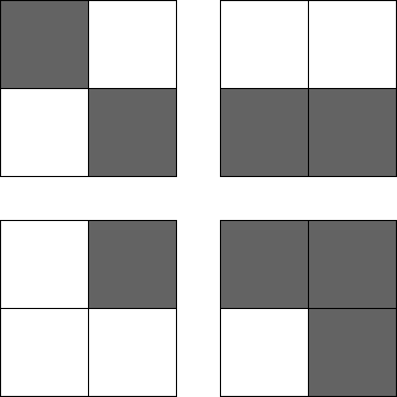
The BUF algorithm is quite clever and is based on the observation that all pixels in a 2x2 block share the same connected component. It's fairly easy to see why. Here are a few examples that cover all possible cases (rotation aside). Dark pixels represent value 1 while white pixels account for value 0. I know, it's well done.

I think that I'm not mistaken by saying that a lot of CCL algorithms lies on a Union-Find data structure under the hood. It is a data structure that keeps track of a collection of disjoint (non-overlapping) sets. It supports two primary operations : Union (which merges two sets into one) and Find (which determines which set a particular element belongs to). This is super useful for efficiently managing connected components, as it allows you to quickly combine groups of connected pixels while keeping track of their identifiers. It works by linking the root of one set to the root of another, ensuring that each element points to a representative member of its set. Here is an example from Wikipedia.

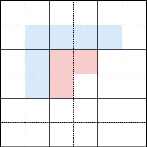
Taking the observation about the blocks into account reduces the initial number of trees by a factor of four (and therefore fewer Union calls). It also decreases the depth of the trees, positively impacting the performance of the Find step. Since we're dealing with blocks, we need to adjust how we define adjacency (while considering the borders, of course). Again, the number of checks to perform is limited. This verification can be done efficiently using bit masks. In the example below, we simply need to check the red pixels of the central block against the blue pixels of the adjacent blocks.

The algorithm is divided into four steps.

1. Initialization : A unique ID is assigned to each block. This step is highly parallelizable as blocks are yet independent.
2. Merging : We merge the IDs of the blocks based on their neighbors. This requires atomic operations and creates dependency trees between the blocks.
3. Compression : We ensure that the root ID of each tree is assigned to every block within that tree.
4. Finalization : We correct any potential background pixels.

Each of these steps uses a dedicated CUDA kernel, with the results stored in global memory. For example, for the initialization step :

__global__ void init(
    const uint8_t *const g_img,
    int32_t *const g_labels,
    const uint32_t w,
    const uint32_t h)
{
    // Each thread basically works on the top-left pixel of a block
    const uint32_t row = 2 * (blockIdx.y * blockDim.y + threadIdx.y);
    const uint32_t col = 2 * (blockIdx.x * blockDim.x + threadIdx.x);
    const uint32_t index = row * w + col;

    // Check for the border of the image
    if ((row >= h) || (col >= w))
    {
        return;
    }

    // The initial index is the raster index (i.e. the ID of the pixel)
    g_labels[index] = index;
}

Because CUDA blocks will run a fixed amound of threads (1024 max.), some will likely work outside the image bounds. Therefore, we need to check if the thread is actually assigned a part of the image (otherwise, we'll get a nice segfault I suppose). I recommend reading the CUDA Tutorial to get more intuition on that.

You can check out the TorchCC code to get more details on the different kernels. I've only introduced the initialization phase, which is pretty straight forward, so everybody can have a glimpse on what's going on.

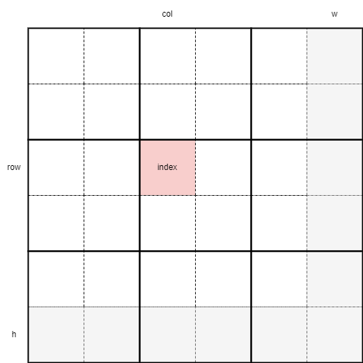
Visually, here's what happens. The gray pixels represent the boundaries of the image (so we can account for edge cases, such as odd dimensions images). Each thread processes a 2x2 pixel block. Please note that I haven't applied any color for 0 or 1 pixels. They're all white. Basically, only the top-left pixel gets assigned an ID.

Next, we define a CUDA grid to execute our various CUDA kernels. Some parameters have been taken from the YACCLAB project, but we could adjust them if needed. In particular, we could set the number of threads per row and per column in the CUDA blocks to 32, with the only limit being a total of 1024 threads per CUDA block. However, by using 16 rows and 16 columns, we can process 4 images in parallel but we'll see this later (well, not exactly 4 images, but a depth of 4 image parts within the batch).

#define BUF_2D_BLOCK_ROWS 16
#define BUF_2D_BLOCK_COLS 16

// [...] Prepare empty labels with PyTorch, extract sizes, do multiple checks, etc.

const dim3 grid = dim3(
    // Working on blocks of 2x2 pixels
    ((w + 1) / 2 + BUF_2D_BLOCK_COLS - 1) / BUF_2D_BLOCK_COLS,
    ((h + 1) / 2 + BUF_2D_BLOCK_ROWS - 1) / BUF_2D_BLOCK_ROWS);
const dim3 block = dim3(BUF_2D_BLOCK_COLS, BUF_2D_BLOCK_ROWS);

init<<<grid, block>>>(mask, labels, w, h);
merge<<<grid, block>>>(mask, labels, w, h);
compress<<<grid, block>>>(labels, w, h);
finalize<<<grid, block>>>(mask, labels, w, h);

Parallezing

The algorithm as described by Allegretti et al. was not designed to be parallelized across multiple images (i.e., to run the algorithm in batches). However, it's quite easy to adapt our implementation to support batch processing. This will reduce the number of instructions sent to the GPU since only 4 kernels will need to be executed, as opposed to a loop that would require 4N kernels to process N images. Consequently, this should also enhance GPU utilization.

The modification needed is quite trivial. We just need to account for the batch depth when calculating the indexes. Each thread will handle one block per image. Of course, we will need to use padding to construct our batch of images. We can use 0 for padding (so padding pixels are considered as background pixels).

__global__ void init(
    const uint8_t *const g_img,
    int32_t *const g_labels,
    const uint32_t w,
    const uint32_t h,
    const uint32_t n)
{
    // Each thread basically works on the top-left pixel of a block in each image
    const uint32_t row = 2 * (blockIdx.y * blockDim.y + threadIdx.y);
    const uint32_t col = 2 * (blockIdx.x * blockDim.x + threadIdx.x);
    const uint32_t depth = blockIdx.z * blockDim.z + threadIdx.z;
    const uint32_t label = row * w + col;
    const uint32_t index = depth * w * h + label;

    // Check for the border of the batch
    if ((row >= h) || (col >= w) || (depth >= n))
    {
        return;
    }

    // Assign a unique ID across the batch (using the raster index would need more careful checks)
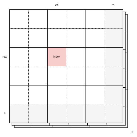
    g_labels[index] = index;
}

Visually, this can be interpreted as follows.

We will also need to adapt how we execute our kernels.

#define BUF_2D_BLOCK_ROWS 16
#define BUF_2D_BLOCK_COLS 16
#define BUF_2D_BLOCK_DEPTH 4

// [...] Prepare empty labels with PyTorch, extract sizes, do multiple checks, etc.

const dim3 grid = dim3(
    // Working on blocks of 2x2 pixels
    ((w + 1) / 2 + BUF_2D_BLOCK_COLS - 1) / BUF_2D_BLOCK_COLS,
    ((h + 1) / 2 + BUF_2D_BLOCK_ROWS - 1) / BUF_2D_BLOCK_ROWS,
    // on each image
    ((n + 1) + BUF_2D_BLOCK_DEPTH - 1) / BUF_2D_BLOCK_DEPTH));
const dim3 block = dim3(BUF_2D_BLOCK_COLS, BUF_2D_BLOCK_ROWS, BUF_2D_BLOCK_DEPTH);

init<<<grid, block>>>(mask, labels, w, h, n);
merge<<<grid, block>>>(mask, labels, w, h, n);
compress<<<grid, block>>>(labels, w, h, n);
finalize<<<grid, block>>>(mask, labels, w, h, n);

Benchmarks

All these GPU stories are nice, but is it really more efficient than what we have on CPU (or the different broken implementations on GPU)? Well, let's find out !

I'll use 50k images of various sizes and densities from the YACCLAB 2D dataset. I'll use the same images for the different benchmarks of course. For each image, I'll save some information, such as the density, the image size (total number of pixels, etc.). I'll run the benchmarks on my machine (i7-12700KF and RTX 3080 Ti).

OpenCV

As OpenCV is not meant to run in a batch fashion, this benchmark ran sequentially on 1 CPU core. Performances could be improved by parallelizing a bit. I used the following script for my benchmark.

torchcc/scripts/benchmark_2d_cpu.py at benchmarks · Bendabir/torchcc

Efficient Connected Components Labeling for PyTorch. - Bendabir/torchcc

GitHubBendabir

On the graph below (mind the logarithmic Y axis), we can observe the impact of the image density and size on the performance. Without much surprise, the bigger the image, the slower the algorithm. The density also impacts the performances as shown by the trendline.

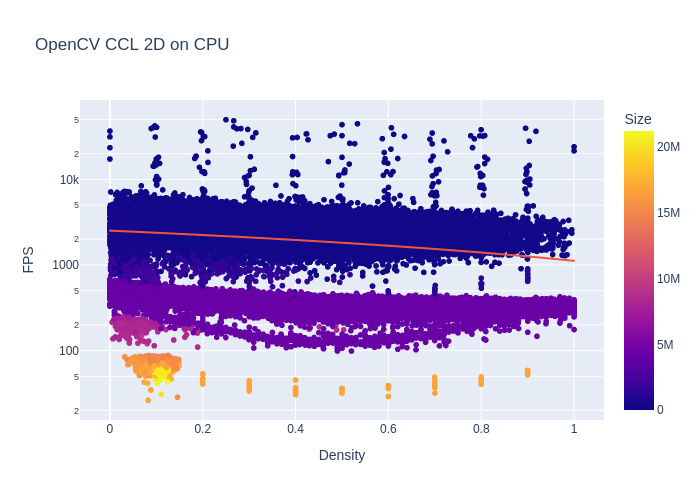
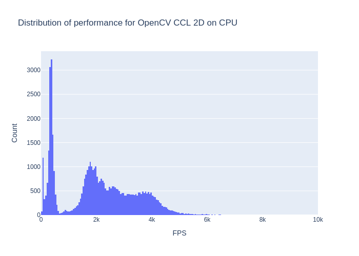
The average performance is 2104 FPS. However, by looking at the performances distribution below (cut at 10k FPS max.) and the graph above, we can easily conclude that it's not really representative. It would probably makes more sense to assess performances for each "class" of images we have (but I've already spent too much time on this).

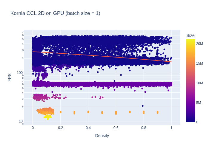
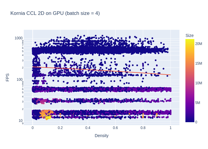
Kornia

I ran a first comparison with batches of size 1 (which is expected to show pretty bad performances). Then I tried with some other batch sizes.

torchcc/scripts/benchmark_2d_kornia.py at benchmarks · Bendabir/torchcc

Efficient Connected Components Labeling for PyTorch. - Bendabir/torchcc

GitHubBendabir

As expected, the implementation is pretty slow. Impact of the density seems to be less pronounced though (mind the logarithmic axis).

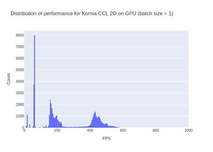
The average performance is 244 FPS. The X axis range is limited to 1k FPS max., so we can see things a bit considering the performances here. Like on the graph above, we observe a similar pattern than the OpenCV implementation regarding performances.

We can observe that we have less correlation between the size and the performances because of the padding we need to use to build the batches. This likely affects the performances because the average performance is now 186 FPS.

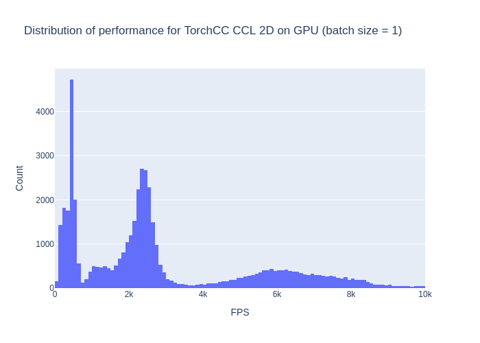
TorchCC

I first run the same benchmark on batch size of 1 for my implementation.

torchcc/scripts/benchmark_2d_cuda.py at benchmarks · Bendabir/torchcc

Efficient Connected Components Labeling for PyTorch. - Bendabir/torchcc

GitHubBendabir

We observe a similar pattern as for the OpenCV implementation, with slightly higher performances.

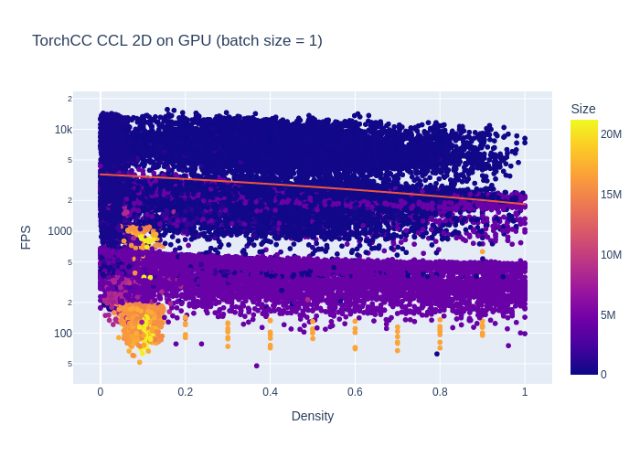
The average performance is 3081 FPS, which is a +46% increase compared to OpenCV. I would have expected more to be honest. However, if we take a look at the distribution, it seems that it's really more efficient overall. Of course, there is room for improvements but we'll discuss that right after !

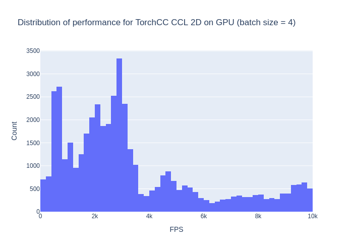
Using batches is favorable here. I start with a batch size of 4.

With batches of size 4, the average performance is 4423 FPS, which is a +110% increase. I'm a bit happier now. Performances are more uniformly distributed.

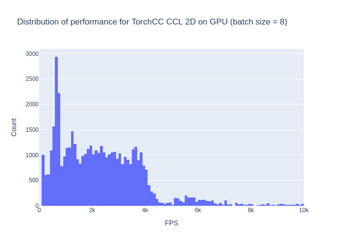
When using bigger batches (size 8 for example), I start to notice a performance drop.

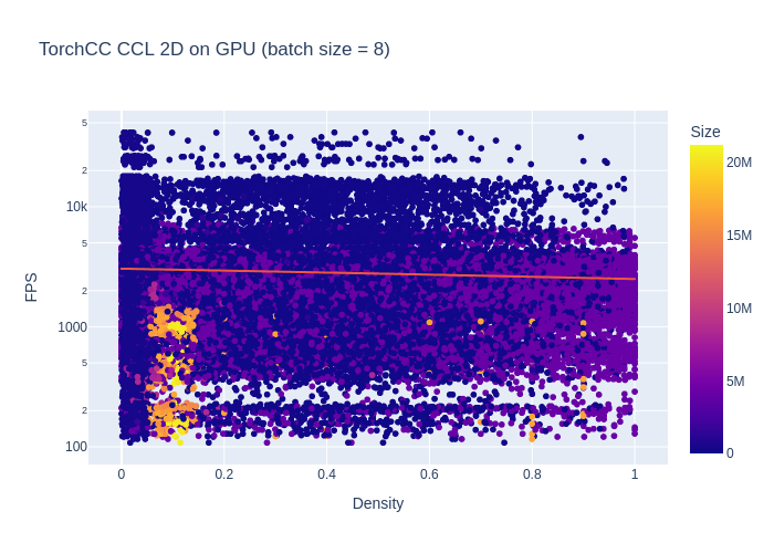
The average performance is now 2882 FPS, which is really close to batches of size 1. It now looks more constrained between 0 and 4k FPS. I would assume that the padding has an impact here. We basically run some extra useless compute on the padding pixels.

If time permits, I'll try to have a look with NVIDIA Nsight Systems so I can better understand what is going under the hood (exact GPU usage, memory transfers, etc.).

Comparison

I'll sum up the previous results in a box plot below.

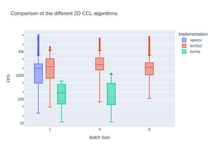
Compared to CPU, we have a 2x performance gain, but there is room for improvements. The major advantage of running CCL on the GPU is that it avoids round trips between the GPU and CPU. When working with an AI model, it's super convenient to handle result decoding directly on the GPU. This eliminates unnecessary data transfers and keeps the processing pipeline efficient.

Going Further

This implementation is just a first draft. There’s still a lot to explore.

To start, it could be interesting to implement BKE, which is slightly more efficient (according to Bolelli et al.). Adapting it for the 3D case (26-connectivity) shouldn’t be too complex either (but we should probably stick to BUF for 3D as suggested by Bolelli et al.).

Currently, only the 8-connectivity case is implemented, but Hennequin et al. seem to offer an interesting approach for 4-connectivity.

Some details still need to be refined. The current implementation of BUF requires contiguous data in memory. As expected, memory access impacts performance (Kerbl et al.). I'm quite convinced that it's possible to enhance the current performance of the algorithm. Perhaps we can avoid some round trips to global memory, which is significantly slower than registers or shared memory. There may be some inspiration to draw from Harris' work. We might also gain some performance on batch padding by using a value other than 0 (like -1 ?), which would eliminate any calculations involving the padding (currently considered background). We saw in the benchmarks that performances degrade when batches are big.

Because we work on blocks of 2x2 pixels, we could compress the input data by representing a block with 1 byte. Each pixel would be encoded with 2 bits. For example :

• 00 : background;
• 01 : foreground;
• 11 : padding (if signed, it represents -1).

I'm not really sure it would be useful though.

Finally, this initial prototype is only compatible with a limited number of CUDA versions (and consequently Python versions). It’s not easy to navigate the various software deprecations. In the future, I would like to keep up with the supported Python versions (at least 3.9 at the time of writing), based on the related PyTorch versions (and thus CUDA). It could also be interesting to provide builds for the few brave souls who run (or worse, develop) on Windows.

References

1. Allegretti, S., Bolelli, F., & Grana, C. (2020). Optimized Block-Based Algorithms to Label Connected Components on GPUs. IEEE Transactions on Parallel and Distributed Systems, 31(2), 423–438. https://doi.org/10.1109/TPDS.2019.2934683
2. Bolelli, F., Allegretti, S., Lumetti, L., & Grana, C. (2024). A State-of-the-Art Review with Code about Connected Components Labeling on GPUs.
3. Hennequin, A., Lacassagne, L., Cabaret, L., Meunier, Q., & Meunier, Q. A. (2018). A new Direct Connected Component Labeling and Analysis Algorithms for GPUs. https://doi.org/10.1109/dasip.2018.8596835ï
4. Harris, M. (2010). Optimizing Parallel Reduction in CUDA
5. Kerbl, B., Kenzel, M., Winter, M. & Steinberger, M. (2022). CUDA and Applications to Task-based Programming