More efficient Connected Components Labeling on GPU

In the previous article, I detailed the first version of TorchCC : a GPU implementation of Connected Components Labeling (CCL) based on the BUF algorithm. It was already faster than a CPU, but I ended with a list of limitations and a will to do better. So here we are.
This article covers TorchCC 0.2.0. The 2D 8-connectivity kernels are about 1.85× faster at batch size 32 (geometric mean over the YACCLAB datasets), and up to 2.8× faster on large document images. Nothing in the algorithm changed. We still do BUF. What changed is how the GPU is fed.
Note
I assume you read the previous article, or at least know what Block-based Union-Find is. In my implementation, the BUF algorithm was split into 4 kernels (init, merge, compress, finalize).
In case you missed it, here’s a short recap. The key idea is to work on 2x2 blocks of pixels. Our kernels do the following things :
init:label[X] = index(X)(each block is a tree)merge:union(X, P/Q/R/S) if connected+ atomicMin (join the trees)compress:label[X] = find(X)inline compression (flatten the trees)finalize: copylabel[X] + 1to the foreground pixels of X (write the output)
Measuring first
Last time, I wrote that we would first need more rigorous measurements to find what to optimize. Nothing big : we cannot blindly optimize or just rely on assumptions. We need to measure to really understand the bottlenecks (either compute or memory), so let’s do that.
In order to understand why a kernel is slow, we need a reference. A labeling must at least read the image (1 byte per pixel) and write the labels (4 bytes per pixel, int32). PyTorch can do exactly that with x.to(torch.int32). I call it the copy bound. It is a realistic lower bound, and everything is expressed as a multiple of it (1.0× is perfect). As this copy does no computation at all, it is only limited by the memory bandwidth : it is our memory bound.
Our test case is the biggest dataset (XDOCS, 3381×5034 pixels) with a batch of 32 images. I chose it for two reasons. First, its images are large (17 Mpx), so a call takes milliseconds : the launch cost is negligible and the timings are stable to a few percent. Second, these are document images, with long text lines and table borders, which make long chains in the Union-Find forest. This is the hard case for the algorithm.
Numbers below come from the same machine as before (RTX 3080 Ti). Processing this batch takes 18.4ms (which is around 5.0× the copy bound, so there is room). Below is the share of time per kernel. The fill kernel is not really one of our kernels but rather a part of the original initialization phase (before the init kernel).
(fill)    █████████████████                   17%
init      ███████████                         11%
merge     ███████████████████████████████████ 35%
compress  ███████████                         11%
finalize  █████████████████████████████       29%
This shows which parts of the algorithm take the most time, and these are the first places to work on. If we become compute bound, there may be nothing more to gain : the GPU is used to its maximum (and, above all, we manage to feed it efficiently). In practice, optimizing the faster parts is less urgent, but it can be a quick win in some cases. The fastest steps may also become the slowest once the other steps are improved.
Tip
GPU timings can be noisy. To compare two builds, I alternate them (old, new, old, new…) and keep the best of a few runs.
Moving fewer bytes
The first fixes are about memory traffic and thread usage. None of them touches the algorithm. We just stop doing useless memory transfers.
The good ideas
1. Do not fill what you overwrite
This one sounds stupid, and it kind of is. The output was allocated with torch::new_zeros, which launches a kernel to write 0 everywhere. However, our finalize kernel writes every pixel anyway (background gets an explicit 0). The pre-fill is pure waste. Replacing it with new_empty removes it. The memory is already allocated by PyTorch and we don’t care about its content. Immediate win : −8% to −17%.
The risk is a pixel that finalize would miss, leaving stale memory. Since the 2x2 blocks tile the image without gaps, even with odd sizes, we are safe (and the tests compare against OpenCV on odd and degenerate shapes).
2. Use the threads we launch
Back in 0.1.0, one CUDA thread block was 16×16×4 threads, with the Z axis used for 4 images. For a single image, 3/4 of the threads exit immediately, but still take scheduler slots. Worse, the grid had one extra Z block when the batch size was a multiple of 4 (see the (n + 1) in the 0.1.0 launch code).
The new layout is 32×8×1 : a warp is exactly one row of 32 consecutive 2x2 blocks (so one contiguous 64-byte segment per pixel row), and each Z slice of the grid is one image. The shape is not random :
- 32 columns is the width of a warp. With 16 columns, a warp covered two half rows, so two 32-byte segments in two different places of the image. Now, each load of a warp is a single contiguous segment.
- 8 rows gives 256 threads per block, which is a comfortable size for the scheduler, and a compact tile of 64×16 pixels. In
merge, the neighborsP,QandRof a block are in the row above. In a tile, they are in the same thread block for 7 rows out of 8. We will see below why this matters.
This also fixes a limit I mentioned last time : the Z dimension of a grid is capped at 65,535. The batch is now processed in chunks of 65,535 images. Each kernel is still a single launch for the whole batch, unless you have more than 65,535 images (so, almost never).
The block scheduler gives work to any SM with free resources, across the whole grid. A 300×300 image only makes about 95 tiles, barely more than one per SM (an RTX 3080 Ti has 80). One launch per image would leave the GPU mostly idle between launches. In a single grid, the tiles of all images fill it together.
I first tried 1D blocks (a strip of 256 threads along a row). It was faster than the old layout, but slower than the 2D tile everywhere. The reason is locality : in merge, a block reads its neighbors above. In a 2D tile, they are mostly in the same thread block (so the same SM, so the same L1). With strips, each vertical link goes through L2. Remember this, locality will come back later.
Result : −15% to −22% at batch size 32, and up to −36% at batch size 1, where 3/4 of the threads were idle. Batch size 1 is not really the target use case, but it’s still nice, so I’ll take it.
3. One label space per image
In 0.1.0, labels were global indices in the batch. That is why N × H × W had to fit in an int32, which limited the batch size. However, images never link together, so a label only needs to be unique inside its image. Each thread now moves its pointers to its own image (with 64-bit offsets) and uses a local index.
No speed change, but no more batch limit (only one image is limited to 2^31 - 1 pixels). This means that we can send bigger batches, which usually means better performance if we manage to feed the GPU correctly. Labels are now unique per image, not across the batch, which makes more sense.
4. A dense buffer for the block labels
This one is the most interesting. BUF stores the label of each block in the output tensor, at the position of the block’s top-left pixel. This is not specific to my implementation. This was actually described in Allegretti et al. [1]. The authors did this to avoid an extra allocation, which at the time meant a slow, synchronizing cudaMalloc. As we interface with PyTorch, which allocates memory for us from a reserved pool, this is less of an issue.
The problem is that GPU memory moves by 32-byte sectors (8 int32). With this layout, only every other int32 of the even rows is a label, and the odd rows hold none :
output tensor (int32), rows r and r+1:

 r   │ L0 │ ·· │ L1 │ ·· │ L2 │ ·· │ L3 │ ·· │   L = block label (top-left pixel), ·· = unused until finalize
 r+1 │ ·· │ ·· │ ·· │ ·· │ ·· │ ·· │ ·· │ ·· │   → 25% of the label memory is useful
So init (which writes) and compress (which reads) each cost about half a full copy for 1/4 of the data, and Find jumps in an array 4× bigger than necessary, which hurts the caches.
As stated before, PyTorch’s caching allocator nowadays makes allocations nearly free after the first call. The reason for the in-place trick is gone. We can use a separate, dense buffer int32[N, ceil(H/2), ceil(W/2)] :
before: labels inside the output                   after: separate dense buffer

 r   │ L0 │ ·· │ L1 │ ·· │ L2 │ ·· │ L3 │ ·· │     │ L0 │ L1 │ L2 │ L3 │ L4 │ L5 │ L6 │ L7 │
 r+1 │ ·· │ ·· │ ·· │ ·· │ ·· │ ·· │ ·· │ ·· │     one sector = 8 useful labels (100%)
For a 1024×1024 image, the working set goes from 4 MB to 1 MB, which now fits in the 6 MB L2 cache of the GPU. Result : −17% to −27% at batch 32. The cost is memory. We now need +1 byte per pixel (from 5 to 6 bytes, so about +20% peak memory). A batch that barely fitted in VRAM may now run out of memory. I think this cost is acceptable. Furthermore, we produce int32 labels, but we could investigate smaller label types (int16, uint8) to reduce the memory footprint (if we can estimate or know ahead the number of labels).
Note
One could argue that we could “store” this buffer inside the output tensor (a bit like a header) to avoid the extra memory cost. However, it’s not as simple. The finalize kernel writes the output while other threads still read block labels. Sharing the same memory would let a thread overwrite a label before another one reads it, as the GPU gives no ordering guarantee inside a kernel.
5. Strides : Do not copy what you can read
The 0.1.0 kernels assumed a contiguous input, so TorchCC copied anything else first. This is a problem for a very common case : a segmentation model outputs one mask per class, as a [N, C, H, W] tensor (C being the number of classes), and we want to label a single class k, so seg[:, k]. This is a view of the model output, not a contiguous tensor, so each call paid for a copy.
A PyTorch tensor is a pointer plus, for each dimension, a stride, which defines how many elements to skip to move by one along this dimension. For our uint8 input, the address of a pixel is :
address(n, r, c) = base + n * sn      + r * sh    + c * sw
                          ▲             ▲           ▲
                          └ next image  └ next row  └ next pixel
A contiguous [N, H, W] tensor has strides (H * W, W, 1), and this is what the old kernels hard-coded (index = depth * w * h + row * w + col, with the neighbors read at offsets of w such as index - w - 1). Two common views break this assumption :
Channel slice: seg is [N, 3, H, W] (C = 3 classes), mask = seg[:, 1]

 memory  │ ch 0 │ ch 1 │ ch 2 │ ch 0 │ ch 1 │ ch 2 │ ...
         ▲                    ▲
         └ image 0            └ image 1 = image 0 + 3*H*W
In mask, the rows of an image are packed (sh = W), but two images are C * H * W apart (sn = 3 * H * W, not H * W), because the other channels sit in between.
Crop: img is [N, H, 8], crop = img[:, :, 2:6]

 row 0 │ . . # # # # . . │
 row 1 │ . . # # # # . . │   pixels of a row are packed (sw = 1),
 row 2 │ . . # # # # . . │   but the next row starts 8 bytes later (sh = 8, while w = 4)
In crop, the pixels kept (#) of a row are still next to each other, but the rows keep the stride of the original image.
The kernels now take sn and sh as parameters (as 64-bit integers, since sn can be huge on a slice of a large batch) instead of assuming index = row * W + col. Only the last dimension must be contiguous (sw = 1). Otherwise, for example with a transpose, the pixels of a row would be spread over memory, every warp load would touch 32 different sectors, and we still copy. The output and the block buffer are allocated by us, so they stay contiguous.
I first estimated the copy at 5% of the call, so not worth it. After the other fixes, the labeling got so much faster that the same copy became a bigger share : on XDOCS ×32, the copy took about 2ms of the 11.9ms call. Result : −15% to −18% on slices, which now cost the same as a contiguous input. This is a good example of something that becomes a new bottleneck once we managed to optimize other parts.
Failed attempt : One thread per pixel in finalize
The finalize kernel is 1.17× the copy bound, which looked improvable. Each thread writes the 4 pixels of its block with 4 stores, and in each store the warp writes with a stride of 2, so each sector is half filled. I thought that I could use one thread per pixel to get consecutive writes and improve performance. Wrong. It was up to 27% slower, and never faster. Two things happened :
- The waste was not real. The “top-right” store fills the other half of the sectors right after the “top-left” one, and L2 merges both writes before they reach DRAM.
- 4× more threads each redo the index math and do 1-byte loads.
Also, finalize cannot reach 1.0× anyway. It reads the image (1 B), the block buffer (about 1 B), and writes the output (4 B) : 6 B instead of 5 B, so a floor of about 1.2×. We measure 1.17×, which is the floor within measurement noise. This kernel is already healthy. We don’t need to try to push it further.
Checkpoint
XDOCS ×32, time per kernel as a multiple of the copy bound

            baseline                                     after
(fill)      █████████████████                   0.84
init        ███████████                         0.53     ████                          0.20
merge       ███████████████████████████████████ 1.75     ███████████████████████       1.14
compress    ███████████                         0.57     █████                         0.27
finalize    █████████████████████████████       1.46     ███████████████████████       1.17
total                                           5.15                                   2.78
These two figures come from two profiling runs, with the GPU in different states. Expressing each kernel relative to the copy bound of the same run removes most of this difference.
With all these improvements, we moved from 18.4ms down to about 9.8ms on XDOCS ×32 (−47%). Ain’t so bad for such “simple” fixes. init and finalize are at their memory bound. However, the merge kernel improved the least. It moves far fewer bytes than finalize, yet takes about as long. It is now the target, and giving it more bandwidth does nothing.
The Slow Horse
I measured it with Nsight Compute, and also with an instrumented build that counts what each thread does. Here is a comparison between merge and finalize on XDOCS (batch 32) :
| Metric | merge | finalize |
|---|---|---|
| DRAM throughput (% of peak) | 22 | 88 |
| L2 throughput (% of peak) | 61 | 16 |
| active threads per warp (out of 32) | 12 | 32 |
finalize is what we want : it (nearly) saturates the memory. merge barely uses DRAM. The data is on chip (84% L1 hits), yet the SMs are busy issuing instructions for few active threads. Half of the time, warps wait for a load.
The reason comes from the Find function (remember the UF algorithm). It is a pointer chase : n = L[n] until L[n] == n. Each load depends on the previous one, so the latency adds up, and no bandwidth can help. The chains can be long, because merge never compresses paths (this is the role of the compress kernel) :
| Case | Redundant Unions | Failed Atomics | Average Hops per Find | Max Hops |
|---|---|---|---|---|
| XDOCS | 64% | 38% | 4.4 | 737 |
| Blobs | 67% | 44% | 2.4 | 40 |
| Noise | 43% | 27% | 1.6 | 28 |
A redundant union is one where both blocks are already in the same tree. We pay for two full Find chains for nothing. This is common in 8-connectivity because links form small cycles :
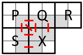
Source: Allegretti et al. [1]
On the previous figure, I’ve identified the connections between blocks : X merges with Q, then with S. P-Q and P-S were already joined by the threads of Q and S, so union(X, S) walks two chains to the same root for nothing.
Each hop is a dependent load. At best, it hits L1 (about 35 cycles). Often, it goes to L2 (about 200 cycles), where all global atomics happen. Shared memory costs about 30 cycles. I found these figures on the NASA website (no kidding, see Basics on NVIDIA GPU Hardware Architecture [4]). They are of course architecture dependent, but they give us a rough idea (and we’re more interested in orders of magnitude here). For L1, let’s consider it a best case figure : L1 is not coherent between SMs, so a hit can return a stale parent, and the walk continues further.
Shared memory      ███                                        ~ 30 cycles
L1 hit             ███                                        ~ 35 cycles
L2 hit             ████████████████████                       ~ 200 cycles
DRAM               ████████████████████████████████████████   ~ 400+ cycles
So what we want is not moving bytes faster, but shorter Find chains in a faster memory. The good news is that, with the 32×8 tiles from before, about 85% of the links of a block stay inside its own tile.
Going local
About fusion
The first question is : why the hell do we have 4 kernels in the first place ? The answer is simple : I used the authors’ implementation as a starting point. Each kernel boundary is a global barrier : all threads of a phase must finish before the next one starts. A phase can be merged into another only if it does not need this barrier (and if we can run both computations without going through the global memory). Don’t get me wrong : their implementation was smart and easy to understand. I’m just trying to push things forward.
The current logic can be represented as follows.
init ─┤ merge ─┤ compress ─┤ finalize
      ▲        ▲           ▲
      │        │           └ Not needed : finalize can call find itself
      │        └ Needed : a root is final only when all unions are done
      └ Needed for global labels, but not for labels inside one tile
We could go further and use a single kernel with a grid-wide barrier (a cooperative launch), but it only saves the launch cost : about 10 to 15 µs per call, which is less than 0.2% of the XDOCS ×32 time. The data would still go through L2 and DRAM between phases because it is shared between SMs. For many tiny calls, a CUDA graph is a better tool. Besides, it would probably be more complicated to program (and I’d like to keep things simple if possible).
Merging compress into finalize
The compress kernel only flattens the trees so that finalize can read the root in one load. We can let finalize find the root itself. This is safe because after merge the forest does not change anymore.
One question that arises is whether to use a plain Find, or a Find with path compression (findAndCompress). The difference is huge on long chains. With plain Find, each of the blocks below a long chain walks all of it. On XDOCS, finalize went from 4.4ms to 6.8ms. With compression, the first threads shorten the path for the others and the time stays at 4.4ms. I kept findAndCompress because I couldn’t identify any bad case.
Result : −3% to −12%, about the time of the old compress kernel plus one launch. Modest, but free.
Union-Find in shared memory
This is the big one. A thread block can synchronize its own threads (using __syncthreads()), so it can run a complete Union-Find on its tile with no global barrier, and in shared memory, but it’s a bit more subtle to program. We replace init + merge with two new kernels :
| Kernel (before) | Operations (before) | Memory (before) | Kernel (after) | Operations (after) | Memory (after) |
|---|---|---|---|---|---|
init | blocks[b] = b | global | localMerge | s[t] = t, union(X, neighbors in the tile), blocks[b] = global index of the tile root | shared |
merge | union(X, P/Q/R/S) | global | borderMerge | union(X, neighbors in another tile) | global |
A tile is 32×8 blocks (64×16 pixels). Only the blocks on the top row and on the left and right columns have a neighbor in another tile : 46 blocks out of 256 (18%).
┌───────────────────────────────────┐
│ T T T T T T T T ... T T T T T T T │   T : P, Q, R are in the tile above
│ L . . . . . . . ... . . . . . . R │   L : P, S are in the tile on the left
│ L . . . . . . . ... . . . . . . R │   R : R is in the tile on the right
│                 ...               │   . : all neighbors in the tile
└───────────────────────────────────┘
It’s a good argument to try doing as much as possible in shared memory. Here is the idea of localMerge, simplified :
__shared__ int32_t s[TILE_H * TILE_W];

s[t] = t;                          // Each block is its own tree

__syncthreads();

for each link of X inside the tile // Same pixel checks as before
    Union(s, t, neighbor);         // atomicMin, but in shared memory

__syncthreads();

blocks[b] = global_index(Find(s, t)); // One coalesced write
Since local and global raster orders are consistent, the tile root is the smallest index of its set, so its global index is never above the block’s one, and the global forest stays acyclic. After this kernel, every tile is flat : each block points directly to its tile root. borderMerge then only needs to join tile roots.
My first borderMerge was almost as slow as the old merge. It used the same grid as the other kernels, and interior threads just returned. However, in each warp, at least 2 lanes out of 32 are on a border, so every warp still ran and the image was almost fully read again. The fix is simple in hindsight : launch only the border threads (46 per tile) and put 4 tiles in a thread block to keep the SMs busy.
The effect on the work done (XDOCS ×32) : global atomics go from 5.7M to 0.5M warp instructions, and global loads from 96M to 31M. The work moved to shared memory.
Global atomics per call (XDOCS ×32)
before  ████████████████████████████████████████████████████████ 5.69M
after   █████                                                    0.54M   (−90%, same for blobs and noise)
Interleaved A/B against the previous step, median, batch 32 :
| Case | Before | After | Gain |
|---|---|---|---|
| Noise | 1 421 µs | 998 µs | −30% |
| Blobs | 1 271 µs | 948 µs | −25% |
| Hamlet | 1 621 µs | 1 289 µs | −21% |
| XDOCS | 9 114 µs | 7 825 µs | −14% |
| Medical | 1 123 µs | 1 003 µs | −11% |
| 3DPeS | 165 µs | 175 µs | +6% |
As predicted by the diagnosis, images with many components gain the most. The loser is 3DPeS, because its images are almost empty (1% foreground). There is no Union-Find work to save, and borderMerge becomes a fixed cost since border blocks read scattered image sectors. It is a trade-off I accept, since about 10 µs on sparse images is not worth worrying about.
I also tried 32×16 tiles (fewer borders). They were 5% to 15% slower : a bigger tile means a longer wait at __syncthreads() for the slowest union. Again, it’s a balance to find.
Benchmarks
Here are some benchmark figures. I used the same setup as in the previous article : Intel i7-12700KF, NVIDIA RTX 3080 Ti, YACCLAB 2D datasets, naive CPU baseline (cv2.connectedComponents in a Python loop). Transfers between CPU and GPU are not included.
On average, TorchCC 0.2.0 is 32.6× faster than the CPU (geometric mean 18.1×), against 8.4× (5.5×) for 0.1.0. However, the two charts come from different runs, and the CPU baseline is noisy, so comparing them overstates the gain. The fair comparison is 0.1.0 against 0.2.0, with the same script, in the same run. Here is the speedup of 0.2.0 over 0.1.0 :
| Dataset | Size | B=1 | B=8 | B=32 | B=64 |
|---|---|---|---|---|---|
| 3DPeS | 576×704 | 0.71× | 1.54× | 1.78× | 1.87× |
| Fingerprints | 300×300 | 1.10× | 1.14× | 1.81× | 1.87× |
| Hamlet | 2125×1273 | 2.00× | 2.23× | 2.23× | 2.76× |
| Medical | 847×1920 | 1.34× | 1.92× | 2.63× | 2.15× |
| MIRflickr | 375×500 | 0.86× | 1.47× | 1.85× | 2.21× |
| Random | 32×32 | 1.00× | 0.79× | 0.77× | 0.88× |
| Tobacco800 | 1575×1200 | 1.68× | 2.12× | 2.27× | 2.26× |
| XDOCS | 3381×5034 | 2.44× | 2.33× | 2.28× | 2.35× |
| Geometric mean | 1.28× | 1.60× | 1.85× | 1.96× |
For instance, XDOCS ×32 went from 19.2ms to 8.4ms. The biggest gains are on large images with a lot of Union-Find work (XDOCS, Hamlet, Tobacco800, Medical), at any batch size. Small images at batch size 1 (3DPeS, MIRflickr) and the random dataset (32×32) are slightly slower than with 0.1.0. They are launch-bound : there is not enough work to feed a GPU, and the extra borderMerge launch costs a few µs. Against the CPU, only random still loses at small batch sizes. That is expected. For such use cases, the right answer is probably a CPU.
The figures for every dataset are in the TorchCC README.
What’s next
Let’s review the limitations I listed in the previous article.
- Warp divergence was partly correct. Tiles removed most of the long chains, but
localMergeis now the largest cost of the merge step. A warp ballot to handle horizontal runs without atomics (HA8-style, Hennequin et al. [3]) is the next candidate. It might be trickier to implement, and I haven’t looked into it yet. - Atomics are mostly fixed. 90% of them now happen in shared memory.
- Block size and Z limit is fixed, with the 32×8 tiles and the chunked batches.
- Contiguity is fixed for the common cases (slices and crops). Only a non-contiguous last dimension still copies. I don’t see any other solution (except different kernels to adapt to this shape maybe).
- Batch size limit has been fixed. The limit now applies to a single image.
There are still some other ideas I have not tried yet : BKE (another algorithm from Allegretti et al. [1], reported as only 1.0 to 1.1× faster than BUF in 2D [1, 2]), keeping the border links computed by localMerge so borderMerge does not read the image again, and full path compression in finalize. Regarding the memory footprint, we might want to produce smaller output types than int32 (int16, uint8, etc.). This would come at the cost of fewer possible labels per image, but that might be a good trade-off in most cases. This could even be the user’s decision.
TorchCC 0.2.0 also brings 4-connectivity and 3D 26-connectivity, which I did not cover here. Maybe a future article, if time (and motivation) allows.
Conclusion
The interesting part of this article and these improvements is that we didn’t really do anything clever. We just took a bit of time to better understand how GPU and memory actually work, and measured the execution to identify pain points. The algorithm is the same. Gains really came from measuring, finding out what the bottleneck really was (bytes first, then latency), and fixing it. Several of my first guesses were wrong (the finalize coalescing, the 1D blocks, the cost of the input copy, etc.), and the profiler was the only reliable judge. The GPU is rarely slow for the reason we think : first measure, then act.
I think the implementation is not yet perfect, and there might be room for improvements (especially on some architectures), but I’m not sure this is the point of the library (and I also have very limited resources to test various architectures).
I don’t really know what my next post will be about, nor when I’ll take time to write something. See you.
References
[1] Allegretti, S., Bolelli, F., & Grana, C. (2020). Optimized Block-Based Algorithms to Label Connected Components on GPUs. IEEE Transactions on Parallel and Distributed Systems, 31(2), 423–438. https://doi.org/10.1109/TPDS.2019.2934683
[2] Bolelli, F., Allegretti, S., Lumetti, L., & Grana, C. (2024). A State-of-the-Art Review with Code about Connected Components Labeling on GPUs. IEEE Transactions on Parallel and Distributed Systems. https://doi.org/10.1109/TPDS.2024.3434357
[3] Hennequin, A., Lacassagne, L., Cabaret, L., & Meunier, Q. (2018). A new Direct Connected Component Labeling and Analysis Algorithms for GPUs. https://doi.org/10.1109/dasip.2018.8596835
[4] Basics on NVIDIA GPU Hardware Architecture. https://www.nas.nasa.gov/hecc/support/kb/basics-on-nvidia-gpu-hardware-architecture_704.html