Behind Blue Eyes - Part 2 : Collecting Data

To answer the question raised in Part 1, we need data on the eye color of lead actors. To my knowledge, no database exists with this information. Wikidata sometimes contains it, but the coverage is very patchy. The simplest and most reliable approach is probably to build an actor dataset, collect their photos, and annotate them. Luckily, that’s exactly what we’re going to do today. The analysis will then follow in a third post.
Source Data
The most well-known data source for movies and TV shows is probably IMDB. The data is very rich, and fortunately IMDB publishes it daily, so no scraping is needed. It is available for non-commercial use at https://datasets.imdbws.com. The dumps used here are dated 2026/04/11. The following files are used :
We extract them with gunzip. To limit memory usage and loading time, a rough first pass filters the relevant lines. It is a bit hacky, but gets the job done.
| |
The files are too large to include here, but filtered versions will be provided later.
Filtering Titles
We are interested in movies and TV shows. Documentaries, animated productions, and similar content will be excluded later. Movies and TV shows are treated separately, as we can expect different actor distributions between the two (and at worst, keeping them separate changes nothing).
We scope the data to 2015-2025, to stay roughly consistent with the baseline study (2016 data, published in 2025). We can expect (hope) there was no major distribution shift over the last 10 years. Perhaps that is something we’ll be able to see in the data though.
We filter for English-language titles from the US region. IMDB does not provide much more detail than that, but this should be a reasonable heuristic. Popularity will help correct for any noise. If we restrict the scope enough, then it will be possible to manually fix remaining issues.
Movies are grouped under titleType "movie" or "tvMovie", and TV shows under "tvSeries" or "tvMiniSeries".
The filters applied are detailed in the notebook 03_extract_titles.ipynb.
Ranking by Popularity
We use vote count as a proxy for viewership. The rating alone is not ideal : the highest-rated film is not necessarily the most watched. Vote count is a better proxy, as more votes generally means more viewers. However, this introduces a bias towards older titles, which have had more time to accumulate votes, so a correction is needed. We compute a popularity score by normalizing vote counts per year (with a lower bound of 0), then retain the top N titles per year.
We can easily see a difference in votes distributions between movies and TV series by simply looking at them. For movies, it seems to be pretty stable over the years, but it would be worth investigating more rigorously.
Looking at the densities directly clearly shows a difference between movies and series. In order to have something readable, the number of votes is plotted on a logarithmic scale.
The rating distributions do differ, confirming the need to keep movies and TV shows separate. We go with 50 movies per year and 25 series per year. There are fewer series, but they span multiple episodes and seasons over several years, which justifies the lower selection count.
Manual Cleaning
A quick manual review of the selected titles confirms the results look reasonable. With 550 movies and 275 series, the full list is manageable to check by hand, and lends itself well to automation with a deep research agent. The goal is to filter out titles with no connection to the US that could introduce bias. The following titles were removed. It might not be perfect but should define a pretty good baseline for our study.
| 12th Fail | Godzilla Minus One | Roma | The Kashmir Files |
| Adipurush | I’m Still Here | RRR | The Killing of a Sacred Deer |
| Aftersun | Jai Bhim | Sadak 2 | The Lobster |
| All Quiet on the Western Front | K.G.F: Chapter 2 | Shershaah | The Platform |
| Anatomy of a Fall | Kantara | Sisu | The Power of the Dog |
| Another Round | Laal Singh Chaddha | Society of the Snow | The Substance |
| Belfast | Last Night in Soho | Soorarai Pottru | The Worst Person in the World |
| Dangal | Late Night with the Devil | Talk to Me | The Zone of Interest |
| Dara of Jasenovac | Napoleon | The Banshees of Inisherin | Train to Busan |
| Dhurandhar | Parasite | The Father | Triangle of Sadness |
| Dil Bechara | Pathaan | The Handmaiden | Yesterday |
| Emilia Pérez | Radhe | The Invisible Guest |
This reduces the dataset from 550 to 503 movies, and from 275 to 211 series. The notebooks 04_filter_series.ipynb and 05_filter_movies.ipynb detail the filtering. The filtered data is available as CSV files: movies_50_us.csv and series_25_us.csv.
Extracting Cast Members
We then extract the actors. For each actor, we count the number of appearances per year, separately for movies and TV shows. Counting each actor once tells you about the casting pool, whether blue-eyed people get hired more, but the intuition behind this study is more visceral : I feel like I keep seeing blue eyes on screen. That’s an exposure question. An actor cast across 15 titles shapes your viewing experience far more than someone who appeared in one film. Weighting by appearances captures this compounding effect, and if blue-eyed actors are also booked more often, that’s a stronger finding than over-representation in the pool alone.
We maintain a separate list for movies and for series, with per-year detail, which will later be used in two ways : aggregated across years as weights in the primary analysis, and broken down per year to test for temporal trends. The full selection process is available in the notebook 06_extract_actors.ipynb. The filtered data is available as CSV files: actors_movies_50_us.csv and actors_series_25_us.csv. The extraction is straightforward : we join our selected titles against the principals data to retrieve the corresponding cast.
Inferring Eye Color
With our actor dataset assembled, the next step is to determine the eye color of each person. Since no structured source provides this information reliably, we resort to visual inference : find a photo for each actor, run it through a vision model, and assign a color category.
Finding Actor Photos
With the actor list in hand, we can look up a photo for each of them and attempt to infer eye color. We use the TMDB API for this as getting images from IMDB is less trivial. Such images are not in the data dumps they provide, and scraping the IMDB website is a bit more complex that simply using a web API. I’d rather not spend my life on this. There are 4,509 unique actors in total (across movies and series). For 282 of them, no photo could be found. A fallback to Wikidata would be possible but unreliable, and rate limiting makes it impractical. The process is straightforward and detailed in the notebook 07_extract_pictures_urls.ipynb.
The real question is what to do with actors for whom no photo is available. Before dropping them, it is worth examining the data to understand the situation better. Missing data in studies like this falls into three mechanisms (which are pretty well covered on Wikipedia) :
- MCAR (Missing Completely At Random) : missingness is unrelated to any variable, observed or not. Safe to just drop and adjust denominators.
- MAR (Missing At Random) : missingness depends on observed variables (billing order, genre, year, ethnicity, etc.) but not on eye color itself. Can correct with weighting or imputation.
- MNAR (Missing Not At Random) : missingness depends on eye color itself. That’s the annoying case.
The analysis below is detailed in the notebook 08_missing_pictures_analysis.ipynb. First, we check whether missingness correlates with billing order and year (the only available covariates), but not with eye color itself. The goal is to determine whether we are in a MCAR, MAR, or MNAR case. A simple logistic regression serves this purpose. If no strong correlation emerges, the data can be considered MCAR and dropping the missing actors is safe. The analysis is run separately for movies and series.
We fit a logistic regression missing ~ ordering + startYear. We then look at a few metrics :
- Pseudo R² measures how much of the variation in missingness the model explains. If its value is close to 0, then the model explains almost nothing. Billing order has a real effect, but missingness is mostly unpredictable noise, which is good news.
- z and P>|z| are from the logistic regression coefficients. The z-score measures how many standard errors the coefficient is from zero. P>|z| is the probability of seeing that z-score by chance if the true coefficient were zero. If p is very small (let’s say smaller than 0.01), then we can assume a real effect of the predictor. If p is big enough (let’s say greater than 0.05), then the effect of the predictor is indistinguishable from noise.
If no predictor is significant and pseudo R² is near 0, missingness is unrelated to observables, meaning MCAR is plausible and it is safe to drop. If ordering or year predicts missingness, we are in the MAR case, which is still safe to drop since missingness depends on observed variables and not on eye color itself.
For movies, there are 3,193 actor entries (spread across multiple years, so duplicates exist) and 253 missing photos (7.9%). The logistic regression results are shown below, with a McFadden pseudo R² of 0.0320 (computed using Python statsmodel package).
| Coefficient | Standard Error | z | P>|z| | |
|---|---|---|---|---|
| Intercept | -54.372326 | 40.922522 | -1.328665 | 1.839585e-01 |
ordering | 0.172923 | 0.023797 | 7.266465 | 3.690157e-13 |
startYear | 0.025098 | 0.020254 | 1.239177 | 2.152800e-01 |
The conclusion is straightforward :
orderingis highly significant (p < 10⁻¹²). Lower-billed actors are more likely to have no picture. This makes complete sense : leads are well-photographed, minor roles aren’t.startYearis not significant (p ≈ 0.22) : no systematic year effect.- Pseudo R² = 0.032. Observables explain very little of the variance in missingness, meaning it’s not strongly structured.
This is textbook MAR : missingness depends on billing order (an observed variable), not on eye color. Dropping actors with no picture is valid. Actors in minor roles are less likely to have photos. This is unsurprising, and not particularly problematic. Lead actors are more prominent and more visible on screen, which is precisely where the original question comes from. For movies, we can therefore safely drop actors with missing photos.
In both cases, billing order is the main driver of missingness. Therefore, actors without photos are dropped.
As an additional safeguard, we will later re-run the primary tests under two extreme scenarios :
- all missing actors assigned
blue/grey, - and all assigned
brown/hazel.
This will help us to confirm the conclusions hold regardless of the missingness mechanism.
We then download the photos for each actor. There is not much to detail, it is simply parallelizing GET requests over a list of URLs. The URLs are available here : actors_urls.csv.
Classifying Eye Color
To annotate the images, I use Gemma 4 E2B (under Apache 2.0 licence). It runs well on a consumer GPU and processes the batches quickly. The model is served with Ollama, which exposes an OpenAI-compatible API. The procedure is detailed in this notebook : 09_classify_eye_color.ipynb.
No model is perfect, and eye color classification is a genuinely ambiguous task. The boundaries between categories like hazel, green, and brown are not always clear-cut, even for a human observer, and image quality or lighting conditions can make things worse. It is therefore important to get an estimate of the model’s error rate, and more specifically to understand the direction of any systematic bias, since not all misclassifications are equally harmful to the analysis.
With so many actors, manually verifying everything is not practical. Instead, we sample a subset for estimation. I asked Claude Sonnet to quickly put together a small annotation app for this purpose. The code is dirty and definitely not maintainable, but it does the job. It’s perfect for a one-shot trashable app. You can see the result in 01_annotation_validation.py.
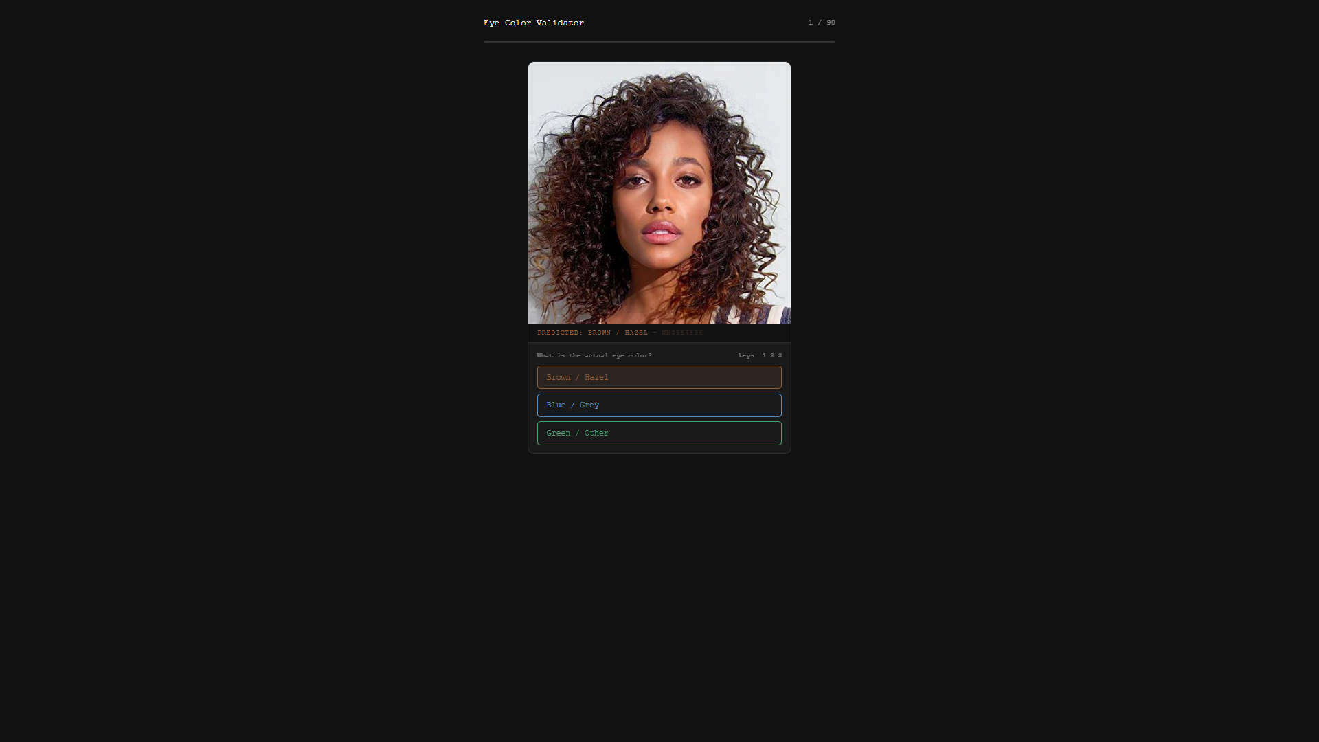
Annotation interface generated by Claude Sonnet
We manually review 90 images (30 per class). The class imbalance is heavy : brown/hazel at 69.1%, blue/grey at 25.7% and green/other at 5.2%.
For validation, stratified sampling is needed, otherwise you would mostly be reviewing brown eyes. It ensures each class gets a fair evaluation (at the cost of an overall accuracy figure that no longer reflects real-world distribution). The images come from the same source and share a similar framing. Stratified sampling at random should therefore yield a representative subset with no obvious subgroup stratification. This gives a good picture of the model’s performance. Stratified sampling is an acceptable tradeoff : per-class accuracy and the confusion matrix are what actually matter for understanding and correcting classifier bias.
Manual annotation took about 5 minutes. Overall accuracy is 97.8% (88/90). One is a clear error : actress nm1409365 is classified as brown/hazel despite obvious blue/grey eyes. The second is debatable : actress nm3908228 is classified as green/other, but depending on the screen, brown/hazel would be equally defensible. It’s a typical boundary case between hazel, brown, and green colors. Excluding it would push accuracy to 98.9%, but the conservative figure is kept. Some images are low quality or dark, making it genuinely hard to distinguish brown from blue in borderline cases.
| Class | Predicted | Truth | Precision | Recall | F1 | Accuracy |
|---|---|---|---|---|---|---|
| Brown / Hazel | 30 | 30 | 96.7% | 96.7% | 96.7% | 96.7% |
| Blue / Grey | 30 | 31 | 100% | 96.8% | 98.4% | 100.0% |
| Green / Other | 30 | 29 | 96.7% | 100.0% | 98.3% | 96.7% |
A few patterns stand out from the results :
blue/grey→brown/hazel: 1 misclassification. The only directionally meaningful error. The classifier occasionally downgrades borderlineblue/greyeyes tobrown/hazel.green/othererrors : 1 misclassification (brown/hazel→green/other), no directional impact onblue/grey.
The single blue/grey → brown/hazel misclassification out of 31 true blue/grey cases (3.2%) means the corpus likely slightly under-counts blue/grey. With blue/grey at 25.7% of the 4,509 actors (~1,159), that translates to roughly 37 expected false negatives (considering that our validation set was representative). The bias is small and conservative : the model will underestimate the proportion of blue/grey actors, so any conclusion reached with these deflated figures would hold equally (or more strongly) against the true proportions. With 30 samples per class, a zero false-positive count should be small enough to be comfortable, but not proof of a perfect classifier.
Overall, the annotations appear trustworthy, though we will account for the uncertainty in the analysis. The annotation results are available here: actors_colors.csv.
Conclusion
We now have a dataset of 713 US English-language titles (503 movies, 211 series) spanning 2015–2025, with eye color annotations for 4,227 out of 4,509 actors. The classifier is reliable, with a small conservative bias on blue/grey : it slightly underestimates the true proportion, which works in favour of a null result. Any finding that survives these deflated figures is the more robust for it. The data is ready. In the next post, we will finally test whether blue-eyed actors are over-represented on screen.