About Connected Components Labeling on GPU

Recently, I read a few things about GPU programming and how it relates to the hardware. It reminded me that a few months ago, I wrote a first draft to do Connected Components Labeling (CCL) efficiently on GPU and interface it with PyTorch: TorchCC. I had almost forgotten this lib existed, but I figured it was a good opportunity to come back to it and explain a bit how it works.
Prologue
Connected Components Labeling
So first off, what is CCL? And more importantly: what is it good for?
When doing text detection in Computer Vision (CV), we may need to use segmentation models. Different approaches exist, but segmentation is one of them. The idea is to assign a class to each pixel of an image. For example: text (foreground) or background. We end up with an image that is “black (1) and white (0)”. This lets us identify the text areas, but not the different text areas. This is what CCL is for: it identifies connected pixels (i.e. pixels that touch each other). If pixels touch, they belong to the same text area. For each area, we assign a different arbitrary label/identifier (a “color”).
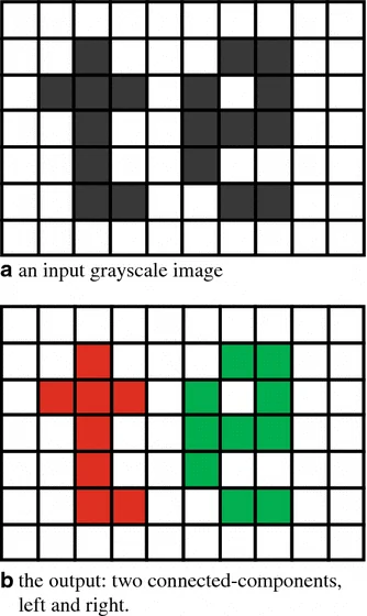
Source: Baek et al. [1]
In fact, this amounts to treating the image as a graph. Of course, CCL is not exclusive to text detection, or even to CV. Still, with an image, the idea is easy to picture.
For an image (so in 2D), there are 2 approaches: 4-connectivity and 8-connectivity. This choice determines how we decide whether two pixels touch:
- 4-connectivity: pixels must share an edge to be neighbors.
- 8-connectivity: pixels must share at least a corner to be neighbors.
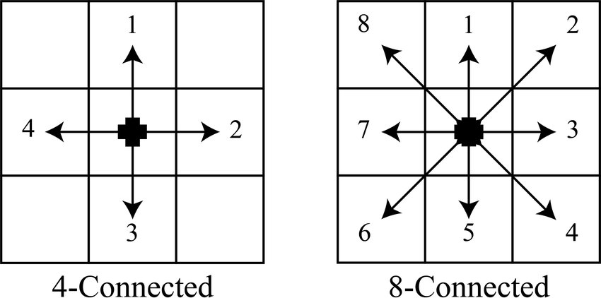
Source: Boundary Fill Algorithm [2]
The choice of connectivity depends on the application domain. There is no good or bad choice.
Once we have assigned a label to each area, we can use it for other applications: image processing, extracting the text area (bounding box, convex hull, etc.). In short, it is usually just an intermediate step.
Unsurprisingly, this generalizes to N dimensions (but that starts to get head-spinning, so let’s keep it simple here).
GPU vs CPU
Alright, all of this is great, but why would we want to run it on a GPU? The reason is fairly simple: an image contains a lot of pixels, and we often want to process many images at once. If we can parallelize per image, we should already see a significant gain over sequential processing on CPU. Luckily, GPUs are very good at parallelizing things (well, if we do it right).
The other argument for an algorithm that would use a GPU efficiently is AI (or any other task running on a GPU, really). Many models can run efficiently on GPU. If we can also do this step on GPU, we potentially save an expensive transfer to the CPU (or even a round trip).
In short, if we manage to do this smartly, it is useful. The good news is that I am not the first to have had this idea, and people much smarter than me have already looked into it.
Introduction
Here, I propose to detail the algorithm used in TorchCC 0.1.0 for 2D 8-connectivity CCL. This version implements the BUF (Block-based Union-Find) algorithm described in Allegretti et al. [3] (and covered in the literature review Bolelli et al. [4]). From what I have seen in the literature on the topic, Union-Find derivatives are a common approach for this kind of problem (and it makes sense, there aren’t many options).
The implementation is written in CUDA (for NVIDIA GPUs) and interfaces natively with PyTorch. Unlike the original implementation of Allegretti et al. [3] (available in the YACCLAB project), which focuses on a single image, it processes batches of images at once (instead of looping). This avoids launching several CUDA kernels (which can slightly affect performance) and makes better use of the GPU. I detail the idea later in the Batching section.
I encourage reading the paper, which I find pretty well done. Here, I will try to explain the general logic and the few edge cases. I will not dwell too much on the exact workings of the GPU, because that would make the article unreadable and a bit long. I may cover that topic later, since there is a lot of room for optimization there.
The basic approach: Union-Find
Before getting into the meat of the topic, I will quickly go over the classic approach to solve this CCL problem. It comes up quite often in the literature, and BUF is just a variant of it.
As we said earlier, we can treat the image as a graph: foreground pixels are nodes, and two touching foreground pixels are linked. A connected component is therefore a group of nodes linked together (directly, or through other nodes). To identify these components, we could simply traverse the graph with a BFS or DFS algorithm. These approaches explore the neighbor graph: starting from a node, we explore every node we can reach, which lets us identify its connected component. Union-Find offers an alternative approach: instead of searching for reachable nodes (neighbors) by traversing the graph, we maintain groups of nodes. If two nodes are neighbors, we merge their groups.
The algorithm
It works as follows. We assign a label to each node. We use an array L that tells us the parent L[i] of node i. A root points to itself (L[i] == i). We could then use this value as the label of the whole connected component. The array L is initialized so that L[i] = i: each node is its own root (i.e. its own connected component).
We then only need 3 operations to identify our connected components:
- Find(a): Walk up the parents until we reach the root.
- Union(a, b): Find both roots, then hang the larger one under the smaller one. Both nodes (and all their groups) are now in the same tree (i.e. same connected component).
- Compress(a): Point
adirectly to its root, so the nextFindcalls only cost a single hop. The following diagram illustrates the idea:
    graph BT
  subgraph after["After Compress"]
    direction BT
    b1((7)) --> r1((0))
    c1((9)) --> r1
    d1((12)) --> r1
  end
  subgraph before["Before Compress"]
    direction BT
    d0((12)) --> c0((9)) --> b0((7)) --> r0((0))
  end
Since we hang the “larger” root under the “smaller” one, the label of a connected component is always its smallest index (so the label is deterministic, which is quite nice).
Application in CCL
Applying this to CCL is quite trivial. We assign a label to each pixel (node). For example: x + WIDTH * y (raster order). This roughly amounts to “flattening” the image. We then apply 2 steps:
- Scan. We go through the pixels in raster order (row by row). For each foreground pixel, we look at its already visited neighbors (depending on the chosen connectivity) and apply
Unionwith those that are foreground. The other neighbors will run the same test on their side later, so each pair is tested only once. - Labeling. For each foreground pixel, we compute its label with
Find(i) + 1(the+1keeps the value0for background). We can also applyCompressto speed up the followingFindcalls.
An example is worth more than a long speech, so here is one with a 4x4 image. I know, it is not a big resolution, but at least we will understand something. We focus here on 8-connectivity (the one implemented in TorchCC). We number the pixels in raster order (so from 0 to 15). For the troublemakers at the back of the class, foreground pixels are marked with the value 1.
image          index
1 1 0 1         0  1  2  3
0 0 1 0         4  5  6  7
0 0 0 0         8  9 10 11
1 0 0 1        12 13 14 15
We initialize L. I intentionally leave the background pixels empty, to keep it readable.
i | 0 | 1 | 2 | 3 | 4 | 5 | 6 | 7 | 8 | 9 | 10 | 11 | 12 | 13 | 14 | 15 |
|---|---|---|---|---|---|---|---|---|---|---|---|---|---|---|---|---|
L[i] | 0 | 1 | 3 | 6 | 12 | 15 |
During the scan phase:
- pixel
1: its left neighbor (0) is foreground, soUnion(1, 0)andL[1] = 0. - pixel
3: no already visited neighbor is foreground, so nothing. - pixel
6: the top-left (1) and top-right (3) are foreground.Union(6, 1)givesL[6] = 0, thenUnion(6, 3)givesL[3] = 0. - pixels
12and15: no foreground neighbors, nothing either.
We end up with the following array L.
i | 0 | 1 | 2 | 3 | 4 | 5 | 6 | 7 | 8 | 9 | 10 | 11 | 12 | 13 | 14 | 15 |
|---|---|---|---|---|---|---|---|---|---|---|---|---|---|---|---|---|
L[i] | 0 | 0 | 0 | 0 | 12 | 15 |
We thus get 3 components with roots 0, 12 and 15 (so labels 1, 13 and 16 to tell them apart from the background).
This is a fairly elegant approach: no queue, no recursion, and the labels pretty much appear on their own. However, this algorithm has a major flaw: the scan is sequential (one pixel at a time), and that is bad for the GPU, which is built for massively parallel computations (and is bad at sequential ones). If we cannot parallelize, we will not do better than the CPU (and maybe even worse).
Block-based Union-Find
Doing one union per pixel is still quite a lot of work. The clever idea behind BUF rests on the following observation (which is only true for 8-connectivity): all foreground pixels in a 2x2 pixel block touch each other (in the 8-connectivity sense). They therefore belong to the same connected component.
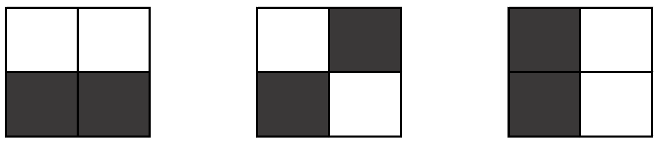
Source: Allegretti et al. [3]
So the idea is not to work on pixels, but on blocks of pixels, in order to reduce the amount of work. Once we have assigned a label to a block, we reuse the block’s label for its pixels. This idea divides the number of nodes to process for the Union-Find algorithm by 4 (and therefore fewer unions). Not bad.
BUF is almost identical to Union-Find, with a few details changed, but we kind of expected that. This algorithm is specifically designed to run on GPU.
1. Nodes are blocks of pixels (rather than single pixels). Each block contains 2x2 pixels. We give it an initial label matching the raster index of its top-left pixel. Two blocks are connected if a foreground pixel in one touches a foreground pixel in the other. As in the “classic” version, we only test neighbors that precede a block in raster order. So for each block X, we only test 4 other blocks: P, Q, R and S.
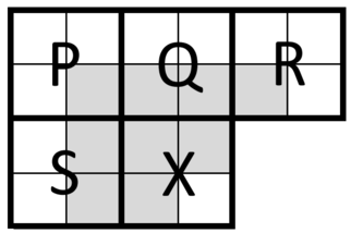
Source: Allegretti et al. [3]
2. Unions are parallel. Sequential unions disappear in favor of parallel unions. Each GPU thread handles one block. All threads work in parallel on the same array L, which raises an obvious problem: concurrent access. The solution proposed by Allegretti et al. [3] is to use atomic operations (atomicMin) to determine the smallest value among the labels. This operation is indivisible: no other atomic operation can modify the same memory address until the previous one has finished. So no write is lost. A root can still change between the moment we find it and the moment we write, but the retry loop below handles that case. Here is the general idea proposed by Allegretti et al. [3]:
// Compiled for the GPU, can only be run on the GPU (but it is not a kernel)
__device__ void Union(int32_t *const L, int32_t a, int32_t b)
{
  bool done = false;

  do
  {
    a = Find(L, a); // Walk up the parents of a to the root
    b = Find(L, b); // Walk up the parents of b to the root

    if (a < b)
    {
      const int32_t old = atomicMin(L + b, a); // Atomically writes min(L[b], a) and returns the old value
      done = (old == b); // Otherwise, someone got there first: we retry
      b = old;
    }
    else if (b < a)
    {
      // Same, but the other way around
      const int32_t old = atomicMin(L + a, b);
      done = (old == a);
      a = old;
    }
    else
    {
      done = true;
    }
  } while (!done); // Keep iterating until we manage to apply the change
}
A few details about this code:
__device__: This qualifier means the function is compiled for the GPU. It can only be called from code already running on the GPU (a kernel or another__device__function), not from the CPU.Find: This is theFindoperation described above. It walks up the parents ofato the root (L[r] == r) and returns that root. Since other threads are modifyingLat the same time, the root we find may no longer be a root by the time we do the union. The loop lets us start over in that case.atomicMin(L + b, a): Atomic operation that writesmin(L[b], a)intoL[b]and returns the old valueold. Ifold == b, thenbwas still a root when we wrote, and the union succeeded. Otherwise, another thread changedL[b]in the meantime. We then continue withb = oldand try again.
As in the classic version, the final root is the smallest index of the component. Using atomic operations lets the threads eventually agree. The rest of the algorithm is identical, except that the operations can be parallelized once all unions are done.
For more details on atomic operations, the Computerphile YouTube channel recently published a video on the topic.
The kernels
That was the general idea. Now, let’s look at the implementation a bit more closely. As we said above, each GPU thread processes one 2x2 pixel block. We define a total of 4 kernels, each of which goes once over the entire image.
init: Each block is its own connected component.merge: Union with the neighboring blocks that touch it.compress: Each block points to its root.finalize: Copy each block’s label into its pixels.
Why use 4 kernels rather than just one? The answer is fairly simple: the dependency between the steps. The merge step needs all blocks to be initialized, and the compress step needs all unions to be finished. Using several sequential kernels provides this synchronization (even though we could do it differently and synchronize threads, but that is a bit more fiddly). Intermediate results go through the GPU’s global memory.
We will look at each kernel in a bit more detail. Remember that each block will be handled by one GPU thread, so each thread will run the kernels (processing its own portion of the image).
1. init
Each block receives its initial label. It corresponds to the (raster) index of its top-left pixel. At this stage, each block is its own component (including the background blocks). Example on a 6x6 image (so 9 blocks):
image                         blocks                  init
┌─────┬─────┬─────┐           ┌───┬───┬───┐           ┌────┬────┬────┐
│ 1 1 │ 0 0 │ 0 1 │           │ A │ B │ C │           │  0 │  2 │  4 │
│ 0 1 │ 0 0 │ 1 0 │           ├───┼───┼───┤           ├────┼────┼────┤
├─────┼─────┼─────┤    ──►    │ D │ E │ F │    ──►    │ 12 │ 14 │ 16 │
│ 0 0 │ 1 0 │ 1 0 │           ├───┼───┼───┤           ├────┼────┼────┤
│ 1 0 │ 0 0 │ 0 0 │           │ G │ H │ I │           │ 24 │ 26 │ 28 │
├─────┼─────┼─────┤           └───┴───┴───┘           └────┴────┴────┘
│ 1 1 │ 0 0 │ 1 1 │
│ 0 0 │ 0 0 │ 1 1 │
└─────┴─────┴─────┘
2. merge
This is the slightly tricky part. Each block X only looks at the 4 neighboring blocks that precede it in raster order: P, Q, R, S. The 4 other neighbors (right and below) do the same check on their side. Each pair of blocks is therefore tested only once.
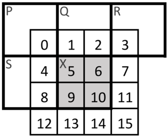
Source: Allegretti et al. [3]
Two blocks are connected if a foreground pixel of X touches a foreground pixel of the neighbor. To avoid re-reading the same pixels, the thread reasons over a 4x4 window around X, numbered from 0 to 15. The pixels we care about are pixels 0, 1, 2, 3, 4 and 8 (in addition to the pixels of X, of course).
Each thread runs 2 sub-steps.
1. Mark. For each foreground pixel of X, we create a mask matching its immediate neighborhood (8-connectivity). Pixel 10 is ignored, it touches neither P, nor Q, nor R, nor S. These masks let us quickly identify the neighboring foreground pixels, through a bitwise & operation.
pixel 5                   pixel 6                  pixel 9
1 1 1 0                   0 1 1 1                  0 0 0 0
1 1 1 0                   0 1 1 1                  1 1 1 0
1 1 1 0                   0 1 1 1                  1 1 1 0
0 0 0 0                   0 0 0 0                  1 1 1 0
Note
The most observant readers will notice that these masks can be computed from the value 0x777 and bit shifts.
2. Check. We combine the masks of the foreground pixels of X (bitwise &). The result tells us which outside pixels we must read: only those among 0, 1, 2, 3, 4 and 8, and only when they are marked. The other pixels of the 4x4 window are never read. For example, with the image below, pixel 5 has only one neighbor: pixel 0 (P). The result also contains pixel 5 itself, which we simply ignore.
image       &     pixel 5     =     neighbors
1 0 0 1           1 1 1 0           1 0 0 0
0 1 0 1           1 1 1 0           0 1 0 0
0 0 0 0           1 1 1 0           0 0 0 0
1 0 0 1           0 0 0 0           0 0 0 0
If a neighbor is identified, we apply Union(X, neighbor) at block level.
| Foreground pixel marked | Union with |
|---|---|
| 0 | P |
| 1 or 2 | Q |
| 3 | R |
| 4 or 8 | S |
A block therefore considers at most 3 of its own pixels and 6 outside pixels, and makes at most 4 unions. The thread stops early in two cases: the mask is empty (pixels 5, 6 and 9 of X are all background), or no marked outside pixel is foreground.
3. compress
After merge, a block may point to a parent that points to another parent, and so on. compress makes each block point directly to the root of its tree. After this step, all blocks of the same connected component carry the same label.
4. finalize
Each thread copies its block’s label (+1, to keep 0 for background) into the 4 pixels of the block. Foreground pixels receive the label, background pixels receive 0. This task is embarrassingly parallel.
Edge cases
So far, we have assumed perfect images, with even sizes and neighbors everywhere. In reality, there are 3 cases that cause trouble (well, 2.5 really).
The borders. A block on the top edge has no P, Q or R. A block on the left edge has no P or S. A block on the right edge has no R. Rather than adding conditions (if statements) when reading the pixels, we adapt the masks generated during the Mark sub-step: we set to 0 the bits that point outside the image (a simple & with a constant, for example 0xEEEE for “everything except column 0”). Since the Check sub-step only reads marked pixels, it never reads outside the image. If everything has been “cleaned”, the mask is empty and the thread stops.
Odd sizes. If the width (or height) is odd, the blocks in the last column (or row) are only one pixel wide (or tall). The pixels in the right column (or bottom row) do not exist: we do not read them, and we also remove from the mask the columns (or rows) that do not exist either. Two situations need to be distinguished:
- the block is in the last column (
col + 1 >= width): it has only one pixel of width, and no neighbor on the right either; - the block is complete but touches the edge (
col + 2 >= width): it has all its pixels, but no column to its right.
Same for rows. In finalize, every write is protected by a bounds check so we never write outside the image.
The worst case. An image where both dimensions are odd: the last block (bottom right) only contains one pixel. Once again, our mask system saves the day. We apply the same two rules as before and everything works out.
Batching
A major difference from the paper is how batches are handled. The reference implementation (available in the YACCLAB repository) only processes one image at a time. To process N images in parallel, we would therefore need to launch our 4 kernels N times. This potentially leads to underusing some warps (groups of 32 threads that execute the same instructions at the same time), and also incurs a scheduling cost for the kernels.
However, we notice that the images are independent of each other. We can therefore use the Z axis of the CUDA grid to identify our images (the X and Y axes are used to locate the pixels).
Warning
blockIdx refers to a block of CUDA threads, not to be confused with our blocks of pixels.
const uint32_t row = 2 * (blockIdx.y * blockDim.y + threadIdx.y);
const uint32_t col = 2 * (blockIdx.x * blockDim.x + threadIdx.x);
const uint32_t depth = blockIdx.z * blockDim.z + threadIdx.z; // The image in the batch
const uint32_t index = depth * width * height + row * width + col; // Pixel index
We only launch our 4 kernels once (well, unless the batch is too big: see the limits below and the Limitations section), and we only do a single allocation for the labels.
An important detail: the labels are the global index within the batch, not the local index within the image. Pixels from two different images are never connected, so the Union-Find trees never mix, and we do not need to check bounds between images. This is convenient, but it has a cost:
N * height * widthmust fit in anint32, which limits the batch size.- From the 2nd image onward, the labels do not start at 1.
- The labels are not contiguous, even in the first image (in the Union-Find example above, we got 1, 13 and 16). If you need labels from
1toK, you must relabel afterward. - All images in the batch must have the same size (or else padding is needed, which amounts to artificially adding background pixels).
Benchmarks
We run a quick benchmark. It is not very rigorous, but it gives an idea of the order of magnitude. We do not take into account the transfer times from CPU to GPU and back. This is not really what interests us here, since the goal is to make CCL possible on data that is already on the GPU.
The benchmark was run on an Intel i7-12700KF and an NVIDIA RTX 3080 Ti, on all the 2D datasets of the YACCLAB project (including randomly generated images). The image dimensions vary, as do the use cases, which should give us a general idea of the performance. The table below gives a typical image size (height × width) for each dataset.
| 3DPeS | Fingerprints | Hamlet | Medical | MIRflickr | Random | Tobacco800 | XDOCS |
|---|---|---|---|---|---|---|---|
576x704 | 300x300 | 2125x1273 | 847x1920 | 375x500 | 32x32 | 1575x1200 | 3381x5034 |
Several batch sizes are tested: 1, 8, 32 and 64. The reference algorithm on CPU is the 2D CCL implementation of OpenCV 4.14, used in a naive way: cv2.connectedComponents is called once per image in a Python loop, with OpenCV’s default thread count.
The gains are significant, even though they vary greatly from one dataset to another. Except for random images at batch sizes 1 and 8, we are always at least as fast as the reference CPU algorithm, even on a single image. These random configurations are unlikely in practice, so we can estimate that we get a significant gain in the general case: between 2× and 20×, depending on the cases and configurations, with a geometric mean gain of around 9×, and a more generous regular mean around 10× (not showed on the graph).
Limitations
This implementation is a good starting point, but it is not perfect. Even though the algorithm is parallel, it is not magic either. We can already identify a few things to improve (which will likely be the subject of another blog post).
- First, it is worth recalling that instructions are executed in parallel in groups of 32 threads, called warps. This means a warp is only as fast as its slowest thread. If some threads finish before others within a warp, resources are wasted. This can happen notably when computing the union step of the BUF algorithm. For example, if a mask is empty, then the thread finishes. Moreover, the number of iterations needed to traverse the components depends on the data, and can vary from one thread to another.
- Using atomic operations can also be problematic. Atomic operations on the same memory location are serialized, so threads that target the same root wait for each other.
- The CUDA block size (not to be confused with our pixel blocks) used by TorchCC (1024) has not been tuned at all, and may be problematic or suboptimal. Moreover, the Z dimension of a CUDA grid is limited to 65535 blocks.
- The current implementation requires the input data to be contiguous, which may require a conversion beforehand.
- The approach for handling batches is imperfect because it limits the number of pixels in a batch. Labels are defined on 4 bytes (
int32) and this range is shared among the images of the same batch, which forces us to artificially limit the batch size so as not to reach the theoretical limit on the number of distinct labels.
It is also likely that some kernels do not make the best use of the GPU’s different memories (shared memory, registers, etc.), but this would require more thorough benchmarking and profiling (which I may do at some point, this lib was mostly a pretext for learning things).
Conclusion
For a first attempt, it is not too bad. We have a 2D 8-connectivity CCL implementation on GPU that shows an average gain of 10× over a CPU implementation. I did not talk about the integration with PyTorch, but it is mostly plumbing and build work, which is a bit outside the scope of this article.
Still, we already see a few limits that suggest we could do better. We therefore need more rigorous measurements to find what to optimize. I have a few ideas in mind, and I may talk about them in a future article.
If time (and motivation) allows, I will try to publish an improved version of the lib (notably by supporting other connectivities and 3D structures).
Cheers.
References
[1] Baek, N., & Kim, K. J. (2017). An artifact detection scheme with CUDA-based image operations. Cluster Computing, 20(1), 749–755. https://doi.org/10.1007/s10586-017-0760-4
[2] OpenGenus IQ. Boundary Fill Algorithm. https://iq.opengenus.org/boundary-fill-algorithm
[3] Allegretti, S., Bolelli, F., & Grana, C. (2020). Optimized Block-Based Algorithms to Label Connected Components on GPUs. IEEE Transactions on Parallel and Distributed Systems, 31(2), 423–438. https://doi.org/10.1109/TPDS.2019.2934683
[4] Bolelli, F., Allegretti, S., Lumetti, L., & Grana, C. (2024). A State-of-the-Art Review with Code about Connected Components Labeling on GPUs. IEEE Transactions on Parallel and Distributed Systems. https://doi.org/10.1109/TPDS.2024.3434357